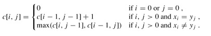
分类: 算法
最长递增子序列(Longest Increasing Subsequence)
最长递增子序列的解法,可以转化为 求最长公共子序列,也就是生成从目标序列从小到大排序之后的新序列,然后计算原始序列与新序列的 最长公共子序列。但是遇到重复数字的时候,会出现问题。也就是这个解法只能解决无重复数字的最长递增子序列。
另外需要注意的就是 最长公共子串(Longest Common Substring)与 最长公共子序列(Longest Common Subsequence)的区别: 子串要求在原字符串中是连续的,而子序列则只需保持相对顺序,并不要求连续。
整个的求解过程其实很好理解:
- 假定要计算的序列为 K = {K1,K2,K3,……,Kn,Kn+1,……,Km}
- 初始化计数数组 N = {N1,N2,N3,……,Nn,Nn+1,……,Nm} ,(计数数组跟序列的长度相同,Kn 的最长递增子序列长度计数对应于 Nn)用来记录最长递增子序列的长度,每个项的初始化值都设置为 1 (即使最小的项,项本身也算一个长度,因此最小的长度是 1)
- 必须从头部(K1)开始遍历
- 当计算 Kn 结尾的最长递增子序列的时候,只要遍历序列 K 的前 [0 ~ n-1] 个项,找到数值 小于(或者小于等于) Kn (必须遍历,Kn 之前的最长递增子序列不一定是 Kn-1 对应的 Nn-1 ),并且在计数数组 N 中对应的计数最大的项 Ni ,然后 Nn = Ni + 1 。
本方法的时间复杂度是 O(n2)
例子:
设数组 K = { 2, 5, 1, 5, 4, 5 } 那么求最长递增子序列的代码如下:
|
1 2 3 4 5 6 7 8 9 10 11 12 13 14 15 16 17 18 19 20 21 22 23 24 25 26 27 28 29 30 31 32 33 34 35 36 37 38 39 40 41 42 43 44 45 46 47 48 |
#include <iostream> #include <vector> int calcMaxLISLength(const std::vector<int>& K) { std::vector<int> N(K.size(), 1); int maxL = 0; for(int i = 0; i < K.size(); i++) { int Ki = K[i]; int maxNi = 0; for(int j = 0; j < i; j++) { int Kj = K[j]; if(Kj < Ki) { int Nj = N[j]; if(Nj > maxNi) { maxNi = Nj; } } } int Ni = maxNi + 1; N[i] = Ni; if(maxL < Ni) { maxL = Ni; } } return maxL; } int main(int argc, char** argv) { // 2 5 1 5 4 5 // 3 std::vector<int> K = {2, 5, 1, 5, 4, 5}; int r = calcMaxLISLength(K); std::cout << r << std::endl; // 17 K = {317, 211, 180, 187, 104, 285, 63, 117, 320, 35, 288, 299, 235, 282, 105, 231, 253, 74, 143, 148, 77, 249, 310, 137, 191, 184, 88, 8, 194, 12, 117, 108, 260, 313, 114, 261, 60, 226, 133, 61, 146, 297, 291, 13, 198, 286, 254, 96, 135, 48, 135, 307, 23, 155, 203, 258, 168, 42, 301, 45, 164, 193, 26, 290, 280, 172, 94, 230, 156, 36, 250, 174, 47, 188, 148, 138, 194, 89, 71, 119, 218, 325, 136, 63, 271, 210, 320, 309}; r = calcMaxLISLength(K); std::cout << r << std::endl; return 0; } |
第二个测试用例的数据如下:
|
1 2 3 4 5 6 7 8 |
输入数据个数 88 实际数据 317 211 180 187 104 285 63 117 320 35 288 299 235 282 105 231 253 74 143 148 77 249 310 137 191 184 88 8 194 12 117 108 260 313 114 261 60 226 133 61 146 297 291 13 198 286 254 96 135 48 135 307 23 155 203 258 168 42 301 45 164 193 26 290 280 172 94 230 156 36 250 174 47 188 148 138 194 89 71 119 218 325 136 63 271 210 320 309 期望结果 17 |
涉及到的面试题目如下类型:
梅花桩问题
合唱队问题
|
1 2 3 4 5 6 7 8 9 10 11 12 13 14 15 16 17 18 19 20 21 22 23 24 |
题目描述 : Redraiment是走梅花桩的高手。Redraiment总是起点不限,从前到后,往高的桩子走,但走的步数最多,不知道为什么?你能替Redraiment研究他最多走的步数吗? 样例输入 6 2 5 1 5 4 5 样例输出 3 提示 Example: 6个点的高度各为 2 5 1 5 4 5 如从第1格开始走,最多为3步, 2 4 5 从第2格开始走,最多只有1步,5 而从第3格开始走最多有3步,1 4 5 从第5格开始走最多有2步,4 5 所以这个结果是3。 输入例子: 6 2 5 1 5 4 5 输出例子: 3 |
合唱队问题
|
1 2 3 4 5 6 7 8 9 10 11 12 13 14 15 16 |
题目描述 计算最少出列多少位同学,使得剩下的同学排成合唱队形 说明: N位同学站成一排,音乐老师要请其中的(N-K)位同学出列,使得剩下的K位同学排成合唱队形。 合唱队形是指这样的一种队形:设K位同学从左到右依次编号为1,2…,K,他们的身高分别为T1,T2,…,TK, 则他们的身高满足存在i(1<=i<=K)使得T1<T2<......<Ti-1<Ti>Ti+1>......>TK。 你的任务是,已知所有N位同学的身高,计算最少需要几位同学出列,可以使得剩下的同学排成合唱队形。 输入描述: 整数N 输出描述: 最少需要几位同学出列 示例1 输入 8 186 186 150 200 160 130 197 200 输出 4 |
合唱队问题其实是 求最长递增子序列 与 最长递减子序列 的 和 最大。
最长递减子序列的求法其实就是把原始序列反序,然后 求最长递增子序列 然后把最后的结果反序即可。
代码如下:
|
1 2 3 4 5 6 7 8 9 10 11 12 13 14 15 16 17 18 19 20 21 22 23 24 25 26 27 28 29 30 31 32 33 34 35 36 37 38 39 40 41 42 43 44 45 46 47 48 49 50 51 52 53 54 55 56 57 58 59 60 61 62 63 64 65 66 67 68 69 70 71 72 73 74 75 76 77 78 79 80 81 82 83 84 85 86 87 88 89 90 91 92 |
#include <iostream> #include <vector> static void calcMaxLIS(const std::vector<int>& K, std::vector<int>& N) { for(int i = 0; i < K.size(); i++) { int Ki = K[i]; int maxNi = 0; for(int j =0; j<i; j++) { int Kj = K[j]; if(Ki > Kj) { int Nj = N[j]; if(maxNi < Nj) { maxNi = Nj; } } } N[i] = maxNi + 1; } } static void calcMaxLDS(const std::vector<int>& K, std::vector<int>& N) { std::vector<int> rK(K.rbegin(), K.rend()); std::vector<int> rN(N); calcMaxLIS(rK, rN); for(int i = 0; i<rN.size(); i++) { N[i] = rN[rN.size() - 1 - i]; } } static int calcMaxVal(const std::vector<int>& K) { std::vector<int> N(K.size(), 1); std::vector<int> rN(K.size(), 1); std::vector<int> KN(K.size(), 0); calcMaxLIS(K, N); calcMaxLDS(K, rN); // /*for(int i = 0; i<N.size(); i++) { std::cout << N[i]; } std::cout << std::endl; for(int i = 0; i<rN.size(); i++) { std::cout << rN[i]; } std::cout << std::endl;*/ for(int i = 0; i<N.size(); i++) { KN[i] = N[i] + rN[i]; } /* for(int i = 0; i<KN.size(); i++) { std::cout << KN[i]; } std::cout << std::endl;*/ int maxL = 0; for(int i = 0; i < KN.size(); i++) { if(maxL < KN[i]) { maxL = KN[i]; } } return maxL - 1; } static void test_calcMaxVal() { std::vector<int> K = {186, 186, 150, 200, 160, 130, 197, 200}; int r = calcMaxVal(K); std::cout << K.size() - r << std::endl; } static void main_test() { test_calcMaxVal(); } static void main_task() { int n = 0; while(std::cin >> n) { std::vector<int> K; for(int i = 0; i<n; i++) { int v = 0; std::cin >> v; K.push_back(v); } int r = calcMaxVal(K); std::cout << n - r << std::endl; } } int main(int argc, char** argv) { //main_test(); main_task(); return 0; } |
解法介绍
|
1 2 3 4 5 6 7 8 9 10 11 12 13 14 15 16 17 18 19 20 21 22 23 24 25 26 27 28 29 30 31 32 33 34 35 36 37 38 39 40 41 42 43 44 |
首先计算每个数在最大递增子串中的位置 186 186 150 200 160 130 197 200 quene 1 1 1 2 2 1 3 4 递增计数 然后计算每个数在反向最大递减子串中的位置--->计算反向后每个数在最大递增子串中的位置 200 197 130 160 200 150 186 186 反向quene 1 1 1 2 3 2 3 3 递减计数 然后将每个数的递增计数和递减计数相加 186 186 150 200 160 130 197 200 quene 1 1 1 2 2 1 3 4 递增计数 3 3 2 3 2 1 1 1 递减计数 4 4 3 5 4 2 4 5 每个数在所在队列的人数+1(自己在递增和递减中被重复计算) 如160这个数 在递增队列中有2个人数 150 160 在递减队列中有2个人数 160 130 那么160所在队列中就有3个人 150 160 130 每个数的所在队列人数表达就是这个意思 总人数 - 该数所在队列人数 = 需要出队的人数 |
参考链接
兔子生兔子问题详解(斐波那契数列)
有一只兔子,从出生后第3个月起每个月都生一只兔子,小兔子长到第三个月后每个月又生一只兔子,假如兔子都不死,问每个月的兔子总数为多少?
斐波那契数列(Fibonacci sequence),又称黄金分割数列、因数学家列昂纳多·斐波那契(Leonardoda Fibonacci)以兔子繁殖为例子而引入,故又称为“兔子数列”,指的是这样一个数列:1、1、2、3、5、8、13、21、34、……在数学上,斐波那契数列以如下被以递推的方法定义:F(1)=1,F(2)=1, F(n)=F(n - 1)+F(n - 2)(n ≥ 3,n ∈ N*)在现代物理、准晶体结构、化学等领域,斐波纳契数列都有直接的应用,为此,美国数学会从 1963 年起出版了以《斐波纳契数列季刊》为名的一份数学杂志,用于专门刊载这方面的研究成果。
这个问题可能我比较笨,看大多数解释都是一句话,f(n) = f(n-1) + f(n-2),但是总有点想不明白这个。列了个表格才看清楚咋回事。
| 月份 | 1 | 2 | 3 | 4 | 5 | 6 | 7 |
| 兔子总数 | 1 | 1 | 2 | 3 | 5 | 8 | 13 |
|---|---|---|---|---|---|---|---|
| 具有生育能力兔子 | 0 | 0 | 1 | 1 | 2 | 3 | 5 |
如果这个月是第n个月,那要求这个月兔子的总数,其实就是上个月的兔子总数加上新生出来的兔子。也就是f(n) = f(n-1) + x。这个x是比较难理解的地方。那这个月到底新生出来多少兔子呢?这就是求这个月已经有生育能力的兔子是多少,上上个月所有的兔子就是这个月所有的有生育能力的兔子,这里可以结合表格推一推就很好理解了。所以x就是f(n-2)。
因此可以得到递推f(n) = f(n-1) + f(n-2)。
其实比较简单的问题,不过自己光凭笨脑子想,突然没想明白,记一下这个思考过程。
还有就是牛客网上的高赞答案详解:
|
1 2 3 4 5 6 7 8 9 10 11 12 13 14 15 |
#include <iostream> using namespace std; int main(){ int m; while(cin>>m){ int a=1,b=0,c=0;//a:一个月兔子数,b:两个月兔子数,c:三个月兔子个数 while(--m){//每过一个月兔子数变化 c+=b; b=a; a=c; } cout<<a+b+c<<endl; } } |
有人是以a表示一个月的兔子,b表示两个月的兔子,c表示三个月的兔子(原文这么注释的),我因为这个注释半天没看懂,后来明白了,c意思是已经成熟的兔子,也就是表示3个月及以上的兔子,也就是说c表示能生兔子的兔子。
那就可以以月份循环,每到达新的一个月,b都会成熟,所以c+=b,c就更新了,仍然表示所有成熟了的兔子,b怎么更新呢?b其实就是上个月那些成熟度是1个月的兔子,所以再更新b,用b=a;a呢?a就是现在更新后的c,因为更新后的c表示这个月成熟了的兔子,那这些兔子都会生一只新的兔子,新兔子就是成熟度为1个月的,所以用a=c。这样现在这个月的兔子总数就是a+b+c。
这是我自己没找到注释,自己总结出来的答案详解,这个方法比递归复杂度低,空间占用更是比用数组先去存要少很多。
参考链接
牛顿迭代法
什么是牛顿迭代法?
牛顿迭代法(Newton's method)又称为牛顿-拉夫逊(拉弗森)方法(Newton-Raphson method),它是牛顿在17世纪提出的一种在实数域和复数域上近似求解方程的方法。
求两个字符串的最长公共子串
问题:有两个字符串str和str2,求出两个字符串中最长公共子串长度。
比如:str=acbcbcef,str2=abcbced,则str和str2的最长公共子串为bcbce,最长公共子串长度为5。
需要注意的就是 最长公共子串(Longest Common Substring)与 最长公共子序列(Longest Common Subsequence)的区别: 子串要求在原字符串中是连续的,而子序列则只需保持相对顺序,并不要求连续。
算法思路:
1、把两个字符串分别以行和列组成一个二维矩阵。
2、比较二维矩阵中每个点对应行列字符中否相等,相等的话值设置为1,否则设置为0。
3、通过查找出值为1的最长对角线就能找到最长公共子串。
针对于上面的两个字符串我们可以得到的二维矩阵如下:
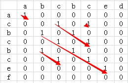
从上图可以看到,str1和str2共有5个公共子串,但最长的公共子串长度为5。
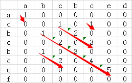
为了进一步优化算法的效率,我们可以再计算某个二维矩阵的值的时候顺便计算出来当前最长的公共子串的长度,即某个二维矩阵元素的值由record[i][j]=1演变为record[i][j]=1 +record[i-1][j-1],这样就避免了后续查找对角线长度的操作了。修改后的二维矩阵如下:
C++代码实现如下:
|
1 2 3 4 5 6 7 8 9 10 11 12 13 14 15 16 17 18 19 20 21 22 23 24 25 |
string getLCS(string str1, string str2) { vector<vector<int> > record(str1.length(), vector<int>(str2.length())); int maxLen = 0, maxEnd = 0; for(int i=0; i<static_cast<int>(str1.length()); ++i) for (int j = 0; j < static_cast<int>(str2.length()); ++j) { if (str1[i] == str2[j]) { if (i == 0 || j == 0) { record[i][j] = 1; } else { record[i][j] = record[i - 1][j - 1] + 1; } } else { record[i][j] = 0; } if (record[i][j] > maxLen) { maxLen = record[i][j]; maxEnd = i; //若记录i,则最后获取LCS时是取str1的子串 } } return str1.substr(maxEnd - maxLen + 1, maxLen); } |
参考链接
快速排序算法(QSort,快排)及C语言实现
上节介绍了如何使用起泡排序的思想对无序表中的记录按照一定的规则进行排序,本节再介绍一种排序算法——快速排序算法(Quick Sort)。
C语言中自带函数库中就有快速排序——qsort函数 ,包含在 <stdlib.h> 头文件中。
快速排序算法是在起泡排序的基础上进行改进的一种算法,其实现的基本思想是:通过一次排序将整个无序表分成相互独立的两部分,其中一部分中的数据都比另一部分中包含的数据的值小,然后继续沿用此方法分别对两部分进行同样的操作,直到每一个小部分不可再分,所得到的整个序列就成为了有序序列。
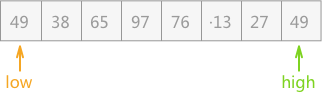
例如,对无序表{49,38,65,97,76,13,27,49}进行快速排序,大致过程为:
- 首先从表中选取一个记录的关键字作为分割点(称为“枢轴”或者支点,一般选择第一个关键字),例如选取 49;
- 将表格中大于 49 个放置于 49 的右侧,小于 49 的放置于 49 的左侧,假设完成后的无序表为:
{27,38,13,49,65,97,76,49}; - 以 49 为支点,将整个无序表分割成了两个部分,分别为
{27,38,13}和{65,97,76,49},继续采用此种方法分别对两个子表进行排序; - 前部分子表以 27 为支点,排序后的子表为
{13,27,38},此部分已经有序;后部分子表以 65 为支点,排序后的子表为{49,65,97,76}; - 此时前半部分子表中的数据已完成排序;后部分子表继续以 65为支点,将其分割为
{49}和{97,76},前者不需排序,后者排序后的结果为{76,97}; - 通过以上几步的排序,最后由子表
{13,27,38}、{49}、{49}、{65}、{76,97}构成有序表:{13,27,38,49,49,65,76,97};
整个过程中最重要的是实现第 2 步的分割操作,具体实现过程为:
- 设置两个指针 low 和 high,分别指向无序表的表头和表尾,如下图所示:
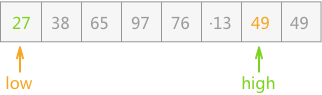
- 先由 high 指针从右往左依次遍历,直到找到一个比 49 小的关键字,所以 high 指针走到 27 的地方停止。找到之后将该关键字同 low 指向的关键字进行互换:
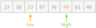
- 然后指针 low 从左往右依次遍历,直到找到一个比 49 大的关键字为止,所以 low 指针走到 65 的地方停止。同样找到后同 high 指向的关键字进行互换:

- 指针 high 继续左移,到 13 所在的位置停止(13<49),然后同 low 指向的关键字进行互换:
- 指针 low 继续右移,到 97 所在的位置停止(97>49),然后同 high 指向的关键字互换位置:
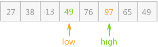
- 指针 high 继续左移,此时两指针相遇,整个过程结束;
该操作过程的具体实现代码为:
|
1 2 3 4 5 6 7 8 9 10 11 12 13 14 15 16 17 18 19 20 21 22 23 24 25 26 27 28 29 30 31 32 33 34 35 |
#define MAX 8 typedef struct { int key; }SqNote; typedef struct { SqNote r[MAX]; int length; }SqList; //交换两个记录的位置 void swap(SqNote *a,SqNote *b){ int key=a->key; a->key=b->key; b->key=key; } //快速排序,分割的过程 int Partition(SqList *L,int low,int high){ int pivotkey=L->r[low].key; //直到两指针相遇,程序结束 while (low<high) { //high指针左移,直至遇到比pivotkey值小的记录,指针停止移动 while (low<high && L->r[high].key>=pivotkey) { high--; } //交换两指针指向的记录 swap(&(L->r[low]), &(L->r[high])); //low 指针右移,直至遇到比pivotkey值大的记录,指针停止移动 while (low<high && L->r[low].key<=pivotkey) { low++; } //交换两指针指向的记录 swap(&(L->r[low]), &(L->r[high])); } return low; } |
该方法其实还有可以改进的地方:在上边实现分割的过程中,每次交换都将支点记录的值进行移动,而实际上只需在整个过程结束后(low==high),两指针指向的位置就是支点记录的准确位置,所以无需每次都移动支点的位置,最后移动至正确的位置即可。
所以上边的算法还可以改写为:
|
1 2 3 4 5 6 7 8 9 10 11 12 13 14 15 16 17 18 19 20 21 22 23 |
//此方法中,存储记录的数组中,下标为 0 的位置时空着的,不放任何记录,记录从下标为 1 处开始依次存放 int Partition(SqList *L,int low,int high){ L->r[0]=L->r[low]; int pivotkey=L->r[low].key; //直到两指针相遇,程序结束 while (low<high) { //high指针左移,直至遇到比pivotkey值小的记录,指针停止移动 while (low<high && L->r[high].key>=pivotkey) { high--; } //直接将high指向的小于支点的记录移动到low指针的位置。 L->r[low]=L->r[high]; //low 指针右移,直至遇到比pivotkey值大的记录,指针停止移动 while (low<high && L->r[low].key<=pivotkey) { low++; } //直接将low指向的大于支点的记录移动到high指针的位置 L->r[high]=L->r[low]; } //将支点添加到准确的位置 L->r[low]=L->r[0]; return low; } |
快速排序的完整实现代码(C语言)
|
1 2 3 4 5 6 7 8 9 10 11 12 13 14 15 16 17 18 19 20 21 22 23 24 25 26 27 28 29 30 31 32 33 34 35 36 37 38 39 40 41 42 43 44 45 46 47 48 49 50 51 52 53 54 55 56 57 58 59 60 61 62 63 64 65 |
#include <stdio.h> #include <stdlib.h> #define MAX 9 //单个记录的结构体 typedef struct { int key; }SqNote; //记录表的结构体 typedef struct { SqNote r[MAX]; int length; }SqList; //此方法中,存储记录的数组中,下标为 0 的位置时空着的,不放任何记录,记录从下标为 1 处开始依次存放 int Partition(SqList *L,int low,int high){ L->r[0]=L->r[low]; int pivotkey=L->r[low].key; //直到两指针相遇,程序结束 while (low<high) { //high指针左移,直至遇到比pivotkey值小的记录,指针停止移动 while (low<high && L->r[high].key>=pivotkey) { high--; } //直接将high指向的小于支点的记录移动到low指针的位置。 L->r[low]=L->r[high]; //low 指针右移,直至遇到比pivotkey值大的记录,指针停止移动 while (low<high && L->r[low].key<=pivotkey) { low++; } //直接将low指向的大于支点的记录移动到high指针的位置 L->r[high]=L->r[low]; } //将支点添加到准确的位置 L->r[low]=L->r[0]; return low; } void QSort(SqList *L,int low,int high){ if (low<high) { //找到支点的位置 int pivotloc=Partition(L, low, high); //对支点左侧的子表进行排序 QSort(L, low, pivotloc-1); //对支点右侧的子表进行排序 QSort(L, pivotloc+1, high); } } void QuickSort(SqList *L){ QSort(L, 1,L->length); } int main() { SqList * L=(SqList*)malloc(sizeof(SqList)); L->length=8; L->r[1].key=49; L->r[2].key=38; L->r[3].key=65; L->r[4].key=97; L->r[5].key=76; L->r[6].key=13; L->r[7].key=27; L->r[8].key=49; QuickSort(L); for (int i=1; i<=L->length; i++) { printf("%d ",L->r[i].key); } return 0; } |
运行结果:
|
1 |
13 27 38 49 49 65 76 97 |
总结
快速排序算法的时间复杂度为O(nlogn),是所有时间复杂度相同的排序方法中性能最好的排序算法。
参考链接
macOS Mojave(10.14.5) Octave libSVM加速SVM计算
|
1 2 3 4 5 6 7 8 9 |
$ cd ~ $ git clone https://github.com/cjlin1/libsvm.git $ cd libsvm $ cd matlab $ octave make.m |
安装完成后,库提供了
svmtrain , svmpredict, libsvmwrite, libsvmread 等函数,可以加速整个 SVM的处理速度。
在 Octave 中使用的方式如下:
|
1 2 3 4 5 6 7 8 9 10 11 12 13 14 15 16 17 18 19 20 21 22 23 24 25 26 27 28 29 30 |
$ octave octave:1> addpath ~/libsvm/matlab octave:2> svmtrain Usage: model = svmtrain(training_label_vector, training_instance_matrix, 'libsvm_options'); libsvm_options: -s svm_type : set type of SVM (default 0) 0 -- C-SVC (multi-class classification) 1 -- nu-SVC (multi-class classification) 2 -- one-class SVM 3 -- epsilon-SVR (regression) 4 -- nu-SVR (regression) -t kernel_type : set type of kernel function (default 2) 0 -- linear: u'*v 1 -- polynomial: (gamma*u'*v + coef0)^degree 2 -- radial basis function: exp(-gamma*|u-v|^2) 3 -- sigmoid: tanh(gamma*u'*v + coef0) 4 -- precomputed kernel (kernel values in training_instance_matrix) -d degree : set degree in kernel function (default 3) -g gamma : set gamma in kernel function (default 1/num_features) -r coef0 : set coef0 in kernel function (default 0) -c cost : set the parameter C of C-SVC, epsilon-SVR, and nu-SVR (default 1) -n nu : set the parameter nu of nu-SVC, one-class SVM, and nu-SVR (default 0.5) -p epsilon : set the epsilon in loss function of epsilon-SVR (default 0.1) -m cachesize : set cache memory size in MB (default 100) -e epsilon : set tolerance of termination criterion (default 0.001) -h shrinking : whether to use the shrinking heuristics, 0 or 1 (default 1) -b probability_estimates : whether to train a SVC or SVR model for probability estimates, 0 or 1 (default 0) -wi weight : set the parameter C of class i to weight*C, for C-SVC (default 1) -v n: n-fold cross validation mode -q : quiet mode (no outputs) |
参考链接
乘积累加运算(Multiply Accumulate, MAC)
乘积累加运算(英语:Multiply Accumulate, MAC)是在数字信号处理器或一些微处理器中的特殊运算。实现此运算操作的硬件电路单元,被称为“乘数累加器”。这种运算的操作,是将乘法的乘积结果和累加器 A 的值相加,再存入累加器:
若没有使用 MAC 指令,上述的程序可能需要二个指令,但 MAC 指令可以使用一个指令完成。而许多运算(例如卷积运算、点积运算、矩阵运算、数字滤波器运算、乃至多项式的求值运算)都可以分解为数个 MAC 指令,因此可以提高上述运算的效率。
MAC指令的输入及输出的数据类型可以是整数、定点数或是浮点数。若处理浮点数时,会有两次的数值修约(Rounding),这在很多典型的DSP上很常见。若一条MAC指令在处理浮点数时只有一次的数值修约,则这种指令称为“融合乘加运算”/“积和熔加运算”(fused multiply-add, FMA)或“熔合乘法累积运算”(fused multiply–accumulate, FMAC)。
积和熔加运算
融合乘加运算的操作和乘积累加的基本一样,对于浮点数的操作也是一条指令完成。但不同的是,非融合乘加的乘积累加运算,处理浮点数时,会先完成b×c的乘积,将其结果数值修约到N个比特,然后才将修约后的结果与寄存器a的数值相加,再把结果修约到N个比特;融合乘加则是先完成a+b×c的操作,获得最终的完整结果后方才修约到N个比特。由于减少了数值修约次数,这种操作可以提高运算结果的精度,以及提高运算效率和速率。
积和融加运算可以显著提升像是这些运算的性能和精度:
积和融加运算通常被依靠用来获取更精确的运算结果。然而,Kahan指出,如果不加思索地使用这种运算操作,在某些情况下可能会带来问题。[1]像是平方差公式x2 − y2,它等价于 ((x×x) − y×y),若果x与y已知数值,使用积和融加运算来求结果,哪怕x = y时,因为在进行首次乘法操作时无视低位的有效比特,可能会使运算结果出错,如果是多步运算,第一步就出错则会连累后续的运算结果接连出错,比如前述的平方差求值后,再取结果的平方根,那么这个结果也会出错。
参考链接
- ^ W.Kahan. IEEE Standard 754 for Binary Floating-Point Arithmetic. May 31, 1996.
- 乘积累加运算
Simple ARM NEON optimized sin, cos, log and exp
This is the sequel of the single precision SSE optimized sin, cos, log and exp that I wrote some time ago. Adapted to the NEON fpu of my pandaboard. Precision and range are exactly the same than the SSE version, so I won't repeat them.
The code
The functions below are licensed under the zlib license, so you can do basically what you want with them.
- neon_mathfun.h source code for sin_ps, cos_ps, sincos_ps, exp_ps, log_ps, as straight C.
- neon_mathfun_test.c Validation+Bench program for those function. Do not forget to run it once.
Performance
Results on a pandaboard with a 1GHz dual-core ARM Cortex A9 (OMAP4), using gcc 4.6.1
command line: gcc -O3 -mfloat-abi=softfp -mfpu=neon -march=armv7-a -mtune=cortex-a9 -Wall -W neon_mathfun_test.c -lm
|
1 2 3 4 5 6 7 8 9 10 11 12 13 14 15 16 17 18 19 20 21 |
exp([ -1000, -100, 100, 1000]) = [ 0, 0, 2.4061436e+38, 2.4061436e+38] exp([ -nan, inf, -inf, nan]) = [ nan, 2.4061436e+38, 0, nan] log([ 0, -10, 1e+30, 1.0005271e-42]) = [ -nan, -nan, 69.077553, -nan] log([ -nan, inf, -inf, nan]) = [ 89.128304, 88.722839, -nan, 89.128304] sin([ -nan, inf, -inf, nan]) = [ nan, nan, -nan, nan] cos([ -nan, inf, -inf, nan]) = [ nan, nan, nan, nan] sin([ -1e+30, -100000, 1e+30, 100000]) = [ inf, -0.035749275, -inf, 0.035749275] cos([ -1e+30, -100000, 1e+30, 100000]) = [ nan, -0.9993608, nan, -0.9993608] benching sinf .. -> 2.0 millions of vector evaluations/second -> 121 cycles/value on a 1000MHz computer benching cosf .. -> 1.8 millions of vector evaluations/second -> 132 cycles/value on a 1000MHz computer benching expf .. -> 1.1 millions of vector evaluations/second -> 221 cycles/value on a 1000MHz computer benching logf .. -> 1.7 millions of vector evaluations/second -> 141 cycles/value on a 1000MHz computer benching cephes_sinf .. -> 2.4 millions of vector evaluations/second -> 103 cycles/value on a 1000MHz computer benching cephes_cosf .. -> 2.0 millions of vector evaluations/second -> 123 cycles/value on a 1000MHz computer benching cephes_expf .. -> 1.6 millions of vector evaluations/second -> 153 cycles/value on a 1000MHz computer benching cephes_logf .. -> 1.5 millions of vector evaluations/second -> 156 cycles/value on a 1000MHz computer benching sin_ps .. -> 5.8 millions of vector evaluations/second -> 43 cycles/value on a 1000MHz computer benching cos_ps .. -> 5.9 millions of vector evaluations/second -> 42 cycles/value on a 1000MHz computer benching sincos_ps .. -> 6.0 millions of vector evaluations/second -> 41 cycles/value on a 1000MHz computer benching exp_ps .. -> 5.6 millions of vector evaluations/second -> 44 cycles/value on a 1000MHz computer benching log_ps .. -> 5.3 millions of vector evaluations/second -> 47 cycles/value on a 1000MHz computer |
So performance is not stellar. I recommend to use gcc 4.6.1 or newer as it generates much better code than previous (gcc 4.5) versions -- almost 20% faster here. I believe rewriting these functions in assembly would improve the performance by 30%, and should not be very hard as the ARM and NEON asm is quite nice and easy to write -- maybe I'll do it. Computing two SIMD vectors at once would also help to improve a lot the performance as there are enough registers on NEON, and it would reduce the dependancies between neon instructions.
Note also that I have no idea of the performance on a Cortex A8 -- it may be extremely bad, I don't know.
Comparison with an Intel Atom
For comparison purposes, here is the performance of the SSE version on a single core Intel Atom N270 running at 1.66GHz
command line: cl.exe /arch:SSE /O2 /TP /MD sse_mathfun_test.c (this is msvc 2010)
|
1 2 3 4 5 6 7 8 9 10 11 12 13 14 |
benching sinf .. -> 1.3 millions of vector evaluations/second -> 303 cycles/value on a 1600MHz computer benching cosf .. -> 1.3 millions of vector evaluations/second -> 305 cycles/value on a 1600MHz computer benching sincos (x87) .. -> 1.2 millions of vector evaluations/second -> 314 cycles/value on a 1600MHz computer benching expf .. -> 1.6 millions of vector evaluations/second -> 244 cycles/value on a 1600MHz computer benching logf .. -> 1.4 millions of vector evaluations/second -> 276 cycles/value on a 1600MHz computer benching cephes_sinf .. -> 1.4 millions of vector evaluations/second -> 280 cycles/value on a 1600MHz computer benching cephes_cosf .. -> 1.5 millions of vector evaluations/second -> 265 cycles/value on a 1600MHz computer benching cephes_expf .. -> 0.7 millions of vector evaluations/second -> 548 cycles/value on a 1600MHz computer benching cephes_logf .. -> 0.8 millions of vector evaluations/second -> 489 cycles/value on a 1600MHz computer benching sin_ps .. -> 9.2 millions of vector evaluations/second -> 43 cycles/value on a 1600MHz computer benching cos_ps .. -> 9.5 millions of vector evaluations/second -> 42 cycles/value on a 1600MHz computer benching sincos_ps .. -> 8.8 millions of vector evaluations/second -> 45 cycles/value on a 1600MHz computer benching exp_ps .. -> 9.8 millions of vector evaluations/second -> 41 cycles/value on a 1600MHz computer benching log_ps .. -> 8.6 millions of vector evaluations/second -> 46 cycles/value on a 1600MHz computer |
The number of cycles is quite similar -- but the atom has a higher clock..
Last modified: 2011/05/29
参考链接
干涉仪测向原理
干涉仪测向原理